Last month I talked about how to use Transpose to copy data from a row and paste it into a column or vice versa. This month we’ll look at a fairly new Excel function ToCol() that can pull data from several adjacent rows and columns and combine it into one column. (There’s also a ToRow() function to combine multiple rows into one.)
Here is how you use this function
=TOCOL(array, [ignore], [scan_by_column])
- Array is simply the range of cells you want to take information from.
- Ignore determines what information, if any, will be ignored. There are four options
0 (or omitted) = Keep all values
1 = Ignore blanks
2 = Ignore errors
3 = Ignore blanks and errors
- Scan_by_column determines whether it reads the data in your array by row or by column.
False (or omitted) = scan by rows
True = scan by columns
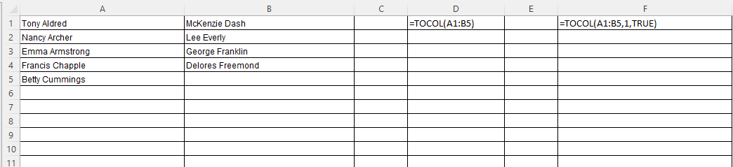
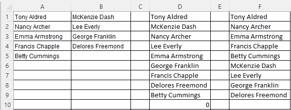
Here’s a simple example. You can see that there are names in columns A and B. In cell D1 is an example of ToCol in its simplest form. Since only an array is specified (A1:B5) Excel assumes the default values for Ignore and Scan_by_column). Then, in F1 is another example using the same array, but setting Ignore to “1” (ignore blanks) and setting Scan_by_column to “True”. In the second picture you can see the results.
Probably the first thing you’ll notice is that we only entered a formula in row 1 of columns D and F, but we have many rows of results. Unlike most Excel functions, ToCol can “spill” results into as many rows as needed.
Both versions of the formula combined the names from the range A1 to B5 (the Array) into one column. Let’s look at the differences in the results.
In column D, we didn’t specify anything for Ignore. The result is that the empty cell from B5, gets displayed as “0” in our list. But in column F, where we set Ignore to 1 (ignore blanks) we only have 9 rows of results instead of the 10 items we have in column D.
In column F, we also set Scan_by_column to True. That is why the names appear in a different order in column D compared to column F. In column D, where we didn’t specify an order, it used the default of reading the array by rows. But in column F, it is reading the array by columns.
Keep in mind that what you see in columns D and F are just the results of the formulas in cells D1 and F1. So they doesn’t behave the same as if those names were there as text. First of all, if the data in the array changes, the results will automatically update. But you can’t highlight the names and click the sort button to sort them. And if you try to copy any of the names other than the top one, and paste it somewhere else, nothing will happen. If you try to copy the first name in either column, you’ll end up copying the formula, not the name.
So how do you turn the results into a list you can use for other purposes? That’s where “Paste Special – Values” comes in. Highlight the cells you want to copy, then click the Copy button on the ribbon (or right-click and choose Copy). Next, right-click where you want your new list, choose Paste Special, then choose Values. The icon will look like this ![]() . Now you’ll have static text instead of a formula and you can work with it like you would any data in Excel.
. Now you’ll have static text instead of a formula and you can work with it like you would any data in Excel.
Do you have trouble remembering how to enter functions like ToCol? Remember that you don’t have to type them directly. The Function Wizard can help you enter your formula correctly with a simple fill-in-the-blank interface


